The representation of meaning

Machine learning (ML) models are functions that map inputs X to outputs Y, no matter how complex such models or domains might seem to be. Although the process of mapping X’s to Y’s varies according to the modeling approach, they all boil down to performing operations and transformations with vectors.

For example, a linear regression model simply computes the inner product between an input vector and a weight vector; tree-based methods work by partitioning the input feature space in useful ways; a feedforward neural network receives an input vector which is multiplied and transformed in cascade by weight matrices and activation functions, respectively.

This discussion may seem abstract at first, but its consequences are very much practical. The takeaway is that to use the ML toolkit off-the-shelf, we need to represent the data we are interested in as vectors.

Fortunately, this is not something we, as ML practitioners, need to worry too much about. In practice, more often than not, the problems that we care about already come with a natural vectorial representation.

Structured data is formatted as a table and by thinking about each row as a feature vector, we can use ML models with no problems. An audio file or other time series are nothing more than long vectors. Images and videos are matrices or tensors, and thus, can be transformed into feature vectors manually or via operations such as convolutions.

Now, think about natural language processing (NLP) for a moment. Words are the foundation of the data used in NLP, but they do not come with a natural vectorial representation like the data types we previously mentioned.

The question then is: how can we represent words (or more generally, text) as vectors so that we can use ML models with them?

It turns out that the answer is not trivial. Up to as recent as 2012, researchers and practitioners used representations that did not capture the nuances present in natural language. However, after 2012, things started changing quickly, to the point that 10 years later (at the time of writing), we have large language models such as BERT, GPT-3, and DALL-E 2 solving awe-inspiring tasks.

Besides hardware advances, the foundation of these results has very much to do with the answer to the question we raised earlier. How to represent words as vectors is what we will explore in this post.

Classical approaches

The classical approach to represent words as vectors is to apply the same rationale that is used to represent categorical features in tabular data: using one-hot vectors.

One-hot vectors are sparse vectors (meaning, having mostly zero elements) that can be used to encode levels. Let’s look at a toy example that will make it clear how they apply to NLP.

Imagine our whole vocabulary had only 5 words: “bottle”, “cat”, “car”, “dog”, and “house”. In this scenario, we could use one-hot vectors with 5 dimensions. The first word in our vocabulary, “bottle”, would be represented as the vector [1, 0, 0, 0, 0]; the second word, “cat”, would be the vector [0, 1, 0, 0, 0]; and so on, until “house”, represented as [0, 0, 0, 0, 1].

Notice that by doing so, each word has a unique vector representation. Furthermore, these vectors would allow us to feed words to ML models. Problem solved, right?

The one-hot encoding approach and variations similar to it were widely used for a long time in the field. However, there are a few issues with it.

The first, and most obvious one, is that languages don’t have only 5 words, but rather millions of words. Consequently, instead of working with 5-dimensional vectors, like in our toy example, models would have to work with sparse and very high-dimensional vectors. Needless to say that finding patterns with such vectors is challenging.

This points straight into another issue with such an approach. At the end of the day, we want models to learn patterns over these word representations and the patterns that we care about in language have a lot to do with similarities and relationships between words. By using one-hot vectors, we are not encoding any notions of meaning or similarity.

The community was well-aware of such limitations and it was not short on efforts that strived to overcome them. For example, circa 2005, Google used to use auxiliary word similarity tables to assess word similarities and improve search results. The problem is that even if we have a vocabulary size of a few hundred thousand words, measuring pair-wise similarities already results in prohibitively large similarity tables.

Word embeddings

Without good representations, learning is doomed to fail, no matter what the modeling approach is. After 2012, a change in how words are represented as vectors led to the astronomical leaps of deep learning on NLP.

Enter the era of word embeddings.

Word embeddings are learned vector representations for words. In contrast to approaches such as one-hot encoding, where the vector representations of words are hand-crafted, word embeddings are learned from data.

As a consequence of the learning process, the resulting vector representations have properties that translate directly to semantic properties that we, as humans, care about.

To make these properties more concrete, let’s look at a few code examples based on GloVe, a popular word embedding method developed at Stanford University.

To do so, the first step is downloading pre-trained word vectors here. For this post, we decided to use 100-dimensional vectors trained on Wikipedia + Gigaword 5, with a vocabulary of 400,000 words, but you can use other available pre-trained vectors as well. We also install the gensim Python module, which is a module for word and text similarity modeling.

After downloading the pre-trained embeddings and installing gensim, we are ready to load the pre-trained word vectors!

from gensim.test.utils import datapath, get_tmpfile
from gensim.models import KeyedVectors
from gensim.scripts.glove2word2vec import glove2word2vec

glove_file = datapath("glove.6B.100d.txt")
word2vec_glove_file = get_tmpfile("glove.6B.100d.word2vec.txt")
glove2word2vec(glove_file, word2vec_glove_file)

model = KeyedVectors.load_word2vec_format(word2vec_glove_file)

The model, above, is a Python dictionary with the words as keys and the corresponding 100-dimensional GloVe vector as value. For instance, if you’d like to check out what the representation would be for the word “banana”, you could simply do:

model["banana"]

Which returns the following 100-dimensional vector:

array([-0.34028  ,  0.46436  , -0.083324 ,  0.20186  , -0.17831  ,
       -0.4663   ,  0.61793  ,  0.30129  ,  0.5728   , -0.34783  ,
       -0.9216   ,  0.30484  ,  0.30382  ,  0.58035  ,  0.12112  ,
        0.77288  ,  1.1547   , -0.576    ,  0.51471  ,  0.21552  ,
        0.21106  ,  0.67875  ,  1.1962   ,  0.11142  ,  0.50809  ,
        1.1873   ,  0.035288 , -0.88952  ,  0.042803 , -0.36714  ,
        0.37993  ,  0.61945  ,  1.0194   , -0.95084  , -0.0072258,
        0.69454  ,  0.38692  , -0.18544  ,  0.2885   , -0.81279  ,
       -0.46473  , -0.82623  ,  0.42778  , -0.14064  ,  0.30173  ,
        0.074418 , -0.40044  ,  0.33969  , -0.62917  , -0.054449 ,
       -0.78469  ,  0.2354   , -0.78359  ,  0.74708  , -0.31074  ,
       -0.07038  , -0.34623  ,  0.33849  ,  0.89621  ,  0.30288  ,
        0.012978 ,  0.020869 , -0.14436  , -0.40914  ,  0.16651  ,
       -0.88124  , -0.078419 ,  0.048156 ,  0.27032  , -0.81761  ,
        0.027778 ,  0.62487  ,  0.1549   , -0.15838  ,  0.088675 ,
        0.063411 , -0.14473  , -0.0066816, -0.18535  ,  1.5642   ,
        0.3726   , -0.81706  , -0.021685 ,  0.91209  , -0.35784  ,
       -0.98389  , -0.37103  , -0.10909  ,  0.18898  , -0.33884  ,
       -0.058326 ,  0.41438  , -1.0411   , -0.42643  , -0.50664  ,
       -0.75863  , -0.15815  , -0.1831   ,  0.7343   , -0.26852  ],
      dtype=float32)

Now we are ready for the interesting part. We can look for the most similar words to the word “banana” by simply doing:

model.most_similar("banana")

The output is:

[('coconut', 0.7097253799438477),
 ('mango', 0.705482542514801),
 ('bananas', 0.6887733936309814),
 ('potato', 0.6629636287689209),
 ('pineapple', 0.6534532308578491),
 ('fruit', 0.6519855260848999),
 ('peanut', 0.6420576572418213),
 ('pecan', 0.6349173188209534),
 ('cashew', 0.6294420957565308),
 ('papaya', 0.6246591210365295)]

Most of them are fruits as well! This is very impressive considering that the computer is answering such queries by navigating the vector space defined by the word embeddings and looking for words associated with similar vectors.

The most surprising example that blew everyone’s minds at the time word embeddings first appeared is related to composability. For example, can add and subtract word embedding vectors to arrive at other words? What happens if we take the vector for the word “king”, subtract the word “man”, then add the word “woman”?

Can you figure out what the answer should be?

It turns out that the answer is “queen”, as one would expect!

model.most_similar(positive=["king", "woman"], negative=["man"])[0]

Here is a simple picture that might help you understand these operations:

This is not a single cherry-picked example. Similar analogies can be found, for example, if we play with nationalities, which indicate that there are directions with meaning in the embedding space. For example, the query:

model.most_similar(positive=["brazilian", "usa"], negative=["brazil"])[0]

Returns “american”.

ML models have a much easier time learning patterns over word embeddings than with one-hot encoded vectors for a few reasons. The first one is that word embeddings are dense and lower-dimensional than one-hot vectors. Note that the dimensionality of the word vectors we used (100) is much smaller than the vocabulary cardinality (400,000), which would not be the case for a lot of the classical approaches. The second is that word embedding vector representations encode notions of similarity and relationship as we saw in the code snippets. Therefore, the vector operations and transformations that ML models explore can be much more fruitful.

The foundation of learning word vector representations from data is an idea from linguistics, called distributional semantics, which coins the notion that similar words often appear together in texts. Therefore, words that are close to each other in texts should be represented by somewhat similar vectors and this serves as a guiding light when learning the vector representations. The details about how the embedding is learned from data are out of the scope of this blog post, but if you are interested, you should check out Stanford professor Christopher Manning’s lecture on the topic.

Using word embeddings for ML model testing

Just to give a practical example of how cleverly constructed word embeddings can be useful in practice, let’s show how they are used at Openlayer to test ML models.

Let’s say that we work at a bank and when clients have questions, they send messages via chat to customer support. You know that the customer support department would benefit greatly from a chatbot to either respond automatically to frequently asked questions or at least to automatically label the kind of inquiry the clients are making so that the messages can be directed to the correct person within the bank.

Equipped with your ML knowledge, you want to train a model that categorizes a client message into a category that represents the kind of question they are making. For example, a message such as “I ordered my card a couple of weeks ago and haven’t received it yet. When can I expect it?” belongs to the class card_delivery_estimate. A message like “Instruct me how to reset the passcode” belongs to the class passcode_forgotten. There are many more classes, as the client’s inquiries can be quite diverse.

However, there is a big challenge hiding in plain sight. The training set has a limited amount of sentences, but clients in the real world can phrase similar inquiries in multiple ways. For example, the sentences “how do I reset my passcode?”, “tell me how to reset my passcode”, and “could you show me how to reset my passcode” all have the same meaning and belong to the class passcode_forgotten, but chances are you don’t have them all in your training set.

How can you prepare your model to handle paraphrases?

If words are represented as embedding vectors, we can find paraphrases by replacing words with others that have close embeddings!

At Openlayer, using invariance tests (which are based on the work of Ribeiro et al. on the CheckList), we can test whether the model’s predictions remain the same even when we paraphrase a sentence. There is a bit more nuance to generating good paraphrases, but the foundational idea is indeed swapping proximal word embeddings. What we often find is that the model is not as robust as expected, so simple paraphrases that are obvious to humans can confuse models.

Here is an example using the chatbot model we described:

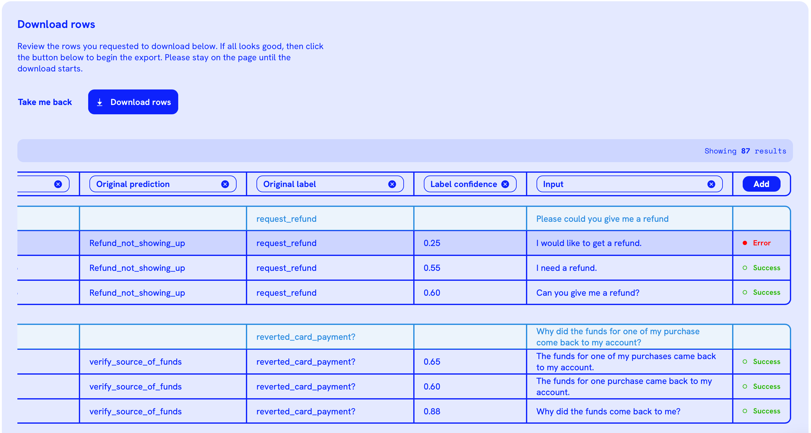
Notice that by simply changing “Please, could you give me a refund” to “I would like to get a refund”, the model starts making mistakes.

Following a data-centric approach, the next logical step would be possibly downloading this synthetic data generated and augmenting the training set to take into account cases where the model exhibits specific failure modes.

The idea of representing words as word embeddings truly transformed the field of NLP. The models currently in use heavily rely on good embeddings to solve tasks from classical sentiment analysis to image generation from text. Hopefully, after reading this post, you are able to appreciate the advances that lay the foundation that pushed the capabilities of ML models to previously unforeseen levels.

* A previous version of this article listed the company name as Unbox, which has since been rebranded to Openlayer.